/case_study_thumb_telit.webp?width=1136&height=639&name=case_study_thumb_telit.webp)


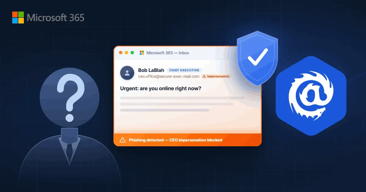
When a Read-Only POC Catches a Live CEO Impersonation Attack
/Leadership%20Headshots/Audian%20Paxson%20Headshot%201000x1000%20032026.webp?width=100&height=100&name=Audian%20Paxson%20Headshot%201000x1000%20032026.webp)
Most email security evaluations are quiet. You connect a tool in read-only mode, let it watch traffic for a few weeks, pull a report, and make a decision. Nobody in the business ever knows it ran.
Read more